Daeus Jorento

Introduction

All models are wrong, but some are useful.
– George E. P. Box

A lot has been written about machine learning (ML), so this is my own study guide. I’m not a machine learning engineer, and I’m not going to get into algorithms here. At a high level, ML is about fitting patterns in data, whether by tracing a curve or drawing a boundary between classifications. For this post, I’m treating the model as mostly a black box.

I like to think of models like a student taking an exam with different strategies. Not studying enough with the material they have is underfitting. Having perfect memory may help on past exams, but fail on the next one when new material shows up, overfitting, or memorizing instead of generalizing. Somehow having the answers beforehand for a practice test is leakage, and will not fly for the real thing. Taking every test the same way as before, even as what is being tested changes, reflects drift.

A truly 100% accurate model is effectively deterministic, which is not realistic for most ML problems. Usually that means you do not need a model, or it is cheating or being evaluated poorly. In general, you reach for ML when heuristics become too complex, though a simple heuristic is often the best place to start.

The hard part of ML is usually not coding the model itself, but everything around it: technical framing, figuring out how the model will actually be used, labeling, cleaning, and feature engineering. After the domain work and data exploration, the final model may look fairly simple. The real difficulty is often in data exploration, ML ops, and offline and online evaluation, including A/B tests.

In practice, ML problems are less about prediction in isolation and more about decision systems. A model is only useful if it changes a downstream business decision or action. The key question is not just “how accurate is the model?” but “what action does this model enable, and what is the cost of being wrong?”

Problem Framing

Two broad types of ML are supervised and unsupervised learning. In supervised learning, we predict an outcome from labeled data, such as revenue or fraud risk. In unsupervised learning, we look for structure in unlabeled data, such as grouping similar cases through clustering. Depending on the problem, the task might be regression, classification, ranking, retrieval, recommendation, or forecasting.

Using the student test analogy, we want the training setup to be as close as possible to the future test. That means giving the student the same information they would actually have, at the same level they would face later.

Where and when will the model be surfaced? Is it triggered by a behavior, run daily in batch, or used some other way? Is it real-time, and if so, how fast does it need to be? We also need to decide the level of prediction: user, page, or specific action.

If the model is real-time, latency matters. In some settings, 10 seconds may be fine. In others, such as recommendations that affect page load time, that would be far too slow. That may require pre-processing or caching rather than live computation.

We may also need to think about cold starts. There is a lifecycle to the model, but also a customer lifecycle that shapes what the model can know and when.

Beyond prediction, it is often helpful to distinguish (e.g. in the setting of fraud detection):

• Prediction: estimating a quantity (e.g., fraud risk);
• Decision: applying a rule or threshold (e.g., block or allow);
• Intervention: what actually happens to the user (e.g., restrict access, require verification).

The unit of prediction (user vs. transaction vs session) is a critical design choice. In many real-world problems, such as fraud detection, the environment is also adversarial, meaning users adapt in response to the system, and the problem itself evolves over time.

Shaping the Data

Ultimately, a model is only as good as the data it trains on. It comes down to inputs and outputs. For LLMs, that often means gathering the right context and iterating on it.

Really, this is often the trickiest part of the work: figuring out the right fit and information. It means doing exploratory data work to find the right features and context, seeing what data we can realistically feed the model, and deciding what the labels are and how we obtain them.

When cleaning up data, we have to make choices about nulls, whether to fill with a mean or median, or drop the data entirely. We may also reduce long-tail categorical data into broader buckets, or convert categorical variables to numeric ones through one-hot encoding.

We might also clip outliers or normalize the data. Another issue is imbalanced data, where rare but important outcomes like fraud require special handling through reweighting or oversampling, such as with SMOTE. A model with 90% accuracy can still be useless if the target class only occurs 1% of the time.

In practice, feature engineering often spans several layers:

• Real-time features (e.g. current transaction details);
• Aggregated real-time / near-real-time features (e.g. activity in the past 24 hours);
• External/vendor features (e.g. third-party data sources);
• Offline features (daily batch pipelines, cached for real-time use).

Those choices involve tradeoffs between feature richness and latency, real-time and cached computation, infrastructure cost and model lift, and freshness and stability.

Labeling is often one of the hardest parts. Labels may be delayed (e.g., fraud realized days later), noisy, or incomplete. Prior models can also influence labels and introduce bias, while proxy labels may differ from the true business outcome. In some cases, it helps to maintain a long-term holdout group without ML intervention so performance can be evaluated against less biased labels.

Model Selection

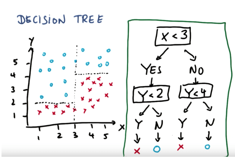
Model selection often depends on the tradeoff between interpretability, flexibility, and performance. In practice, regressions, decision trees, XGBoost, neural nets, Naive Bayes, and other approaches all have their place depending on the structure of the problem and the data. Some methods, such as SVMs, XGBoost, and neural nets, can also take more tuning and experimentation. Autoresearch can be a useful first pass.

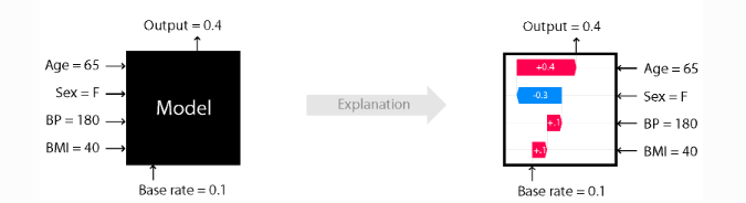
If interpretability matters, simpler models may be easier to explain, though tools like SHAP can help explain feature contributions in more complex models. If we need explainability, such as for revenue predictions that affect sales compensation, we may want to keep the features clear and reduce complexity unless the added lift is worth it. More complex models can also overfit, becoming less flexible in new situations. Regularization can help by penalizing model complexity, trading a bit more bias for less variance. Bias comes from overly simple or wrong assumptions, while variance comes from sensitivity to small changes in the data.

In many real-world problems, feature quality matters more than model choice. Tree-based methods often perform well on structured data because they are flexible and robust. More complex models can improve performance, but they also raise tuning costs, increase overfitting risk, and slow iteration cycles.

Offline Evaluation

Offline evaluation is where much of model development happens. For simplicity, the examples below focus mostly on binary classification, using metrics such as accuracy, precision, recall, F1 score, and AUC.

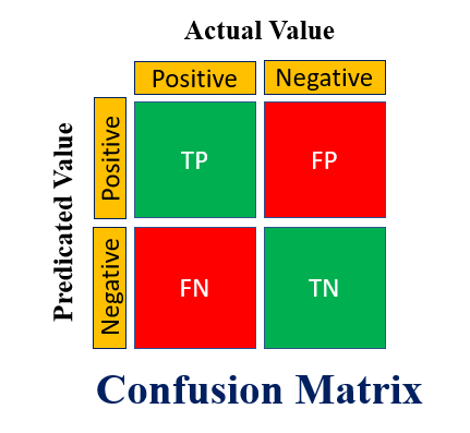
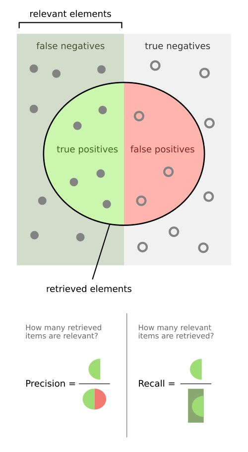
• Confusion Matrix: true positives (TP), true negatives (TN), false positives (FP), false negatives (FN);
• Accuracy: share of all predictions that are correct: (TP + TN) / (TP + TN + FP + FN);
• Precision: share of positive predictions that are correct: TP / (TP + FP);
• Recall: share of actual positives that we catch: TP / (TP + FN);
• F1 score: harmonic mean of precision and recall: 2 × (Precision × Recall) / (Precision + Recall).

In regression or forecasting contexts, metrics such as MAE, MSE, MAPE, and forecast bias are also useful.

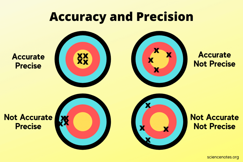
For classification, models often output probabilities, and we can set different thresholds to classify our target groups. For example, I can get 100% recall by labeling everything positive, but then precision will be very low. Or I can set a very high threshold and get strong precision, but miss many true positives.

• Precision-Recall (PR) curve: the tradeoff between precision and recall across different thresholds.
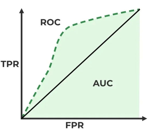
• Receiver Operating Characteristic (ROC) curve: the tradeoff between the True Positive Rate (TPR, or sensitivity) and the False Positive Rate (FPR, or 1 – specificity).
  • X-axis: False Positive Rate (FPR), or the share of actual negatives incorrectly labeled positive.
  • Y-axis: True Positive Rate (TPR), or the share of actual positives correctly labeled positive.
• Area Under the Curve (AUC): the area under the ROC curve.
  • AUC ranges from 0.5 to 1.0, where 0.5 is random guessing and 1.0 is perfect separation.
  • Note: We can also look at Area Under PR curve for imbalanced problems.

For recommendation systems, a common evaluation metric is Mean Reciprocal Rank (MRR). The reciprocal rank is the inverse of the rank of the first correct answer: 1 for first place, 1/2 for second, 1/3 for third, and so on. The mean is the average of those reciprocal ranks. This lets us value getting the right answer second over getting it third, even if we did not get it first.

When doing offline analysis, we often split our sample into train, evaluation, and test sets. Train is where the model learns its parameters. Evaluation is where we compare models or tune inputs. Test is the final offline check. Sometimes people just use train and test, since we still will not know how the model performs in production until it ships.

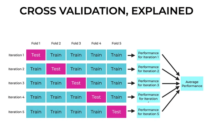
A simple train-test split might be 70/30, but that can be noisy if the test set happens to contain unusual outliers or edge cases. One way to reduce that risk is k-fold cross validation. There, we split the data into k groups, train on all but one, test on the remaining group, and repeat that process across all groups. This gives a better sense of how the model performs across the full dataset (and gives more reliable estimates for errors), rather than relying on one split.

When we split the data, we may do so by customer, action, timestamps, or something else. Again, we want the setup to reflect the actual production situation as closely as possible. In practice, time-based splits are often more realistic than random splits.

Usually the balance is between overfitting, where the model memorizes noise and has high variance, and underfitting, where the model is too simple and has high bias. That is the bias-variance tradeoff: over- or under-shooting complexity.

Offline metrics often do not translate directly to business impact. In many cases, evaluation should reflect cost asymmetry (e.g. for false positives vs. false negatives), use domain-specific metrics rather than generic ones, and mimic production conditions as closely as possible.

For example, recall may be weighted by financial loss, and precision may be defined in terms of business outcomes rather than pure classification correctness. Label contamination from prior models can also bias evaluation, making it important to use global holdout groups when possible.

Online Reality

For online evaluation, the question is more like: how well would this model do tomorrow if it shipped today? Often this means testing in shadow mode before launch to make sure the model is actually doing what we expect. A/B testing is also useful afterward, since we want to measure real impact and lift over the baseline while checking guardrails and segment-level performance. Offline performance, or even improved accuracy metrics, does not always translate to real-world impact or business value.

To set this up, we need proper logging and observability. First, we need to confirm that things are actually working, that the model version matches what we expect, and that the scale looks right. Once things go live, we need monitors for bugs, drift, latency, and other issues. 

We have to evaluate the model based only on what we would actually know at the time of the decision. That means building feedback loops to catch issues quickly and keep improving the model. Those loops help us spot leakage, drift, stale proxy labels, and other failure modes. They also help us see whether offline gains survive launch. Some models improve overall but still hurt key subgroups, and may need to be split or handled differently. Threshold selection also becomes a business optimization problem, balancing competing objectives. In many cases, thresholds may vary across segments, such as users with higher or lower expected lifetime value.

To reduce noise in online experiments, techniques such as triggered analysis can focus on affected users rather than the entire population.

ML deployment is fundamentally about tradeoffs, not just model improvements. In fraud, for example, the real question may involve balancing fraud loss reduction, revenue impact, and operational cost. Segment-level analysis is often required, since the impact of errors can vary across user groups.

We need monitoring not just on the model, but on upstream inputs as well. Models are also often iterated on continuously as we keep trying to improve them. Non-technical stakeholders also need to understand how things are performing and what weeks or months of investment actually produced. In some cases, we want a clean fallback if the model fails, so things do not become catastrophic.

For LLM systems especially, it can also help to run ablation tests, removing one part of the setup at a time to see how much each component actually contributes, since outputs can be less deterministic.

Monitoring and Iteration

Once deployed, models require continuous monitoring and iteration. We need to track input feature distributions, output score distributions, performance metrics over time, and operational signals like latency and system health.

Models can also change user behavior, creating feedback loops that alter future data. In adversarial settings like fraud, this effect can be especially strong. Logging the actual features used at inference time is also critical for ensuring consistency between training and production data.

Models are rarely static. They are updated continuously as new data, signals, and failure modes emerge.

Wrap up

In practice, ML is less about fancy math and more about practical judgment:

• What are you optimizing, and for whom?
• Can the model be explained and trusted?
• Does it help someone make a better decision?

Strong ML practitioners also spend a lot of time on tradeoff analysis, system design, and organizational alignment. The hard part is often in thinking through improvements and iterations, much of which stays hidden in the final product.

Another tricky part is not overselling. No model is ever truly 100% accurate, even with perfect context in many cases. In fraud, fraudsters adapt. In prediction, unexpected shocks like COVID can always happen. The real story is usually more complex, with stakeholders, tradeoffs, and business pressure all falling on the production model owner.

ML is one tool among many. In some cases, product changes, heuristics, or process improvements may be more effective solutions. The real complexity lies in iteration, deployment, and long-term maintenance. The final model may look simple, but the path to getting there, and keeping it working, is where most of the work happens.

Thanks Rob Wang for the review and contributions!