Daeus Jorento

Diagnosing a Slow Query

This is a living document. If you know me or we’re connected on LinkedIn and spot something wrong or missing, please reach out. If I learn something new and update the post, I’ll credit you.

Introduction

Data! Data! Data!…I can’t make bricks without clay.
– Arthur Conan Doyle (Sherlock Holmes: The Adventure of the Copper Beeches)

Anyone who has worked with data will eventually encounter a query that runs and runs. What is the SQL actually asking the database to do? What makes a large table slow to query or build? Why doesn’t making a model incremental always solve the problem?

I recently had an incremental data model begin slowing down and putting downstream workflows at risk as it grew. While the company growth behind it was a good thing, the slowdown felt like a good reason to return to the basics of data modeling and query performance, especially as I use AI to write more of my code and work in unfamiliar domains.

Data engineering is the broader practice of ingesting, moving, storing, transforming, and serving data reliably. This post focuses on one part of that system: analytical data modeling inside and around the warehouse. I am primarily covering table structure, transformations, pipelines, and query performance from the perspective of a data scientist who builds and uses these models, rather than an engineer operating the entire data platform.

How I Learned Data

I loved numbers for a long time, mostly through math and swim statistics, but I didn’t work seriously with data until after college. At the Federal Reserve, I helped manage databases and handle new data releases. At SoFi, I was introduced to SQL.

We had been working with CSVs and dashboards when I finally gained access to the underlying Postgres and MySQL databases. I learned reactively. When something didn’t work, I would get frustrated, discover I had the wrong tool or assumption, and add something new to my toolkit.

Very early on, I ran SELECT * FROM big_table to see what was inside a table. One day, I did this on a massive daily snapshot of every loan at the company. I quickly received a message from the database administrator on HipChat (no, not Slack): “NO, stop that.” He shamed me in the channel, then disappeared to fix something else when I asked what I should do instead.

Someone else suggested starting with a small sample, such as SELECT * FROM big_table LIMIT 2. This was one of the first times I thought about what my SQL was physically asking the database to do. Until then, I had mostly taught myself by validating data in Excel, recreating the same work in SQL, and gradually taking on more complicated questions. As a side note, PGExercises or SQLzoo are great resources for learning basic SQL commands.

Today, I might start by looking for existing documentation or asking someone who has worked with the table before. Then I would describe it, sample a few rows, and review queries that other people have written. More recently, I have used AI to explore unfamiliar tables, although it is mostly performing these same steps and can only work with the context it receives. Its effectiveness depends on the data setup and how clearly the tables, columns, and relationships are named and documented.

Ad hoc requests taught me to clarify the question before touching the data. If someone asked for “customers with a credit score above 750 and a loan above $5,000,” I had to ask what they meant and what they intended to do with the data. Did they want the latest credit score? Open loans or every loan in the customer’s history? Once the definitions were clear, I could narrow down the tables, validate a few known cases, check the joins, and ship the result.

We couldn’t create temporary tables on my team at the time at SoFi, so every query had to be self-contained. That pushed me toward Common Table Expressions, or CTEs, as the questions became more complicated.

At Square, I encountered much larger payments datasets and began building production ETLs and data models. I used temporary tables to validate each stage locally, then converted the logic into reusable models. I learned how upstream dependencies determine when a table can run and how incremental models avoid rebuilding an entire history every day. Sometimes the question itself required a lot of data, such as measuring payments churn across the entire user base and company history.

Square also taught me that different kinds of data require different guarantees. When I gave new hires an overview of the company’s data, I would ask which type they would want to make 100% correct. Eventually, they would settle on payments. The actual movement of money had to add up. Strong financial data followed downstream, with carefully structured definitions for payment volume, interchange fees, merchant categories, and financial reporting.

Eventstream data was much messier. Originally, every click and view across web, mobile, and other surfaces flowed into one massive table. Over time, it was split into more specific tables and eventually migrated into a customer data platform with customizable events available in real time.

There are only two hard things in Computer Science: cache invalidation and naming things.
– Phil Karlton

Once the infrastructure improved, naming and coordination became harder. Different product teams had different incentives and definitions, but their events occupied shared spaces. A name like product_launch might make sense to one team while becoming meaningless across dozens of products. Adding event logging taught me to distinguish data needed for analytics, debugging, and monitoring potential risks. It also taught me how often two sources can disagree because they refresh at different times or define the same concept differently.

I noticed that analysts joining unfamiliar teams would sometimes build a small personal data mart at a grain they understood, such as one row per user, business, or day. At first, I relied heavily on established tables such as dim_user and dim_business. Clean, source-of-truth tables like these are common at mature companies but much less so at startups. Later, I came to appreciate these smaller data marts. Reproducing basic totals by day or business is a practical way to validate my assumptions before attempting anything more complicated.

More recently, I used AI much more heavily to explore and structure data. It made execution faster, but I spent most of the time validating the tables and checking that I was operating from sound premises. I could produce results quickly while understanding the underlying models less deeply.

This was my formal education in data modeling: almost entirely practice, with little theory. I learned by answering business questions, breaking things, validating the results, and building models for product launches, monitoring dashboards, and recurring analysis. This post is my attempt to work backward from those experiences and better understand what the database is actually doing, especially when a table becomes large and slow.

The Grain of the Table Is the Grain of the Question

Data interviews taught me to start with the grain: what does one row represent? Common grains include an event, transaction, user, business, or day. They can also combine, such as one row per user per day. Most of my career has involved loans, payments, and transactions, but the same principle holds across domains. Fact tables usually record events or measurements, dimensions describe entities, and snapshots capture their state at a particular time. Dimensions can also preserve changes over time, often by creating a new row whenever an entity’s attributes change (known as an SCD).

Choosing the grain means choosing which questions the table should answer. A data engineer might prioritize reusable structures that work across the warehouse, while an analyst or data scientist might build more directly around recurring business and product questions. More detail preserves more possible uses, but it also increases storage, complexity, and the work required to query the table. Some data costs much more than the value it provides.

This same tension appears when deciding what a startup needs from its first data hire: is the immediate constraint unreliable infrastructure or unanswered business questions?

Time makes grain more complicated. The same record might have an event time, ingestion time, creation time, and completion time, sometimes across multiple time zones. Data can arrive late, refresh in real time or daily, and be corrected after it first appears. A table should make clear which timestamp and state each row represents.

Shared dim_date and dim_report_period tables map each date to calendar or fiscal weeks, months, and quarters. This reduces duplicated logic and makes it easier to roll the same data up to a different time grain.

A schema organizes this constellation of tables, usually with a tradeoff between simplicity and duplication. One big table can make a known analysis simple and fast, but it often duplicates data and becomes difficult to maintain. A star schema keeps measurements in fact tables and descriptive attributes in dimension tables, making common analytical queries relatively straightforward. A snowflake schema further normalizes those dimensions, reducing duplication but requiring more joins. Highly normalized operational data can be easy to update but cumbersome to analyze.

Every model also determines which information survives. Aggregating transactions to one row per user per day makes many queries faster, but removes the individual transaction details. If an event was never logged, no later model can recover it. This is part of why AI struggles with data. Code may show what a function does, but the usefulness of a data model depends on definitions, questions, and context that may not appear in the SQL.

Rows, Columns, and Joins

Once data has been ingested and organized, we can query it ad hoc or schedule transformations that feed dashboards, ML systems, and other data models. Upstream data infrastructure focuses on reliably collecting and storing data. Downstream work shapes that data for particular uses. Both are constrained by compute, cost, freshness, and maintenance.

At a high level, query cost depends on how much data the engine must read and what it must do afterward. Rows, columns, and data types determine how much data exists. Filters determine how much can be skipped. Joins, aggregations, and sorts determine how much work happens after the initial scan.

All else equal, more rows require more work. Still, row count alone is a weak measure of size. An Excel worksheet stops at 1M rows, while a SQL table can contain billions. The SQL table can still answer some questions much faster because the database does not need to display every row. It can read only the necessary data, process it in parallel, and return a small result. Calculating one total across a billion rows is very different from returning a billion rows.

Columns work similarly. Core tables often accumulate hundreds of columns over time, but that does not mean every query must read all of them. In a columnar warehouse, a query that selects five columns can often skip the other 95. Data types also matter. Repeated booleans and categories generally compress well, while long strings and large JSON objects contain much more information. This is why SELECT * can become expensive even when the row count stays the same.

Joins introduce another dimension: cardinality, or how many rows match each row on the other side. With a left join, a one-to-one or many-to-one match should preserve the starting row count. An inner join can remove unmatched rows, while a many-to-many join (e.g. cross join) can multiply them (Cartesian product). Null keys usually do not match, while duplicate keys can create unexpected fanout.

Joining on too few columns is a common interview mistake. If two tables contain one row per user per day, joining only on user_id matches every date on one side to every date on the other. This creates more rows, not more columns. The query then has to carry those rows through later aggregations, sorts, and joins. Validating key uniqueness and checking row counts before and after a join catches many of these problems. 

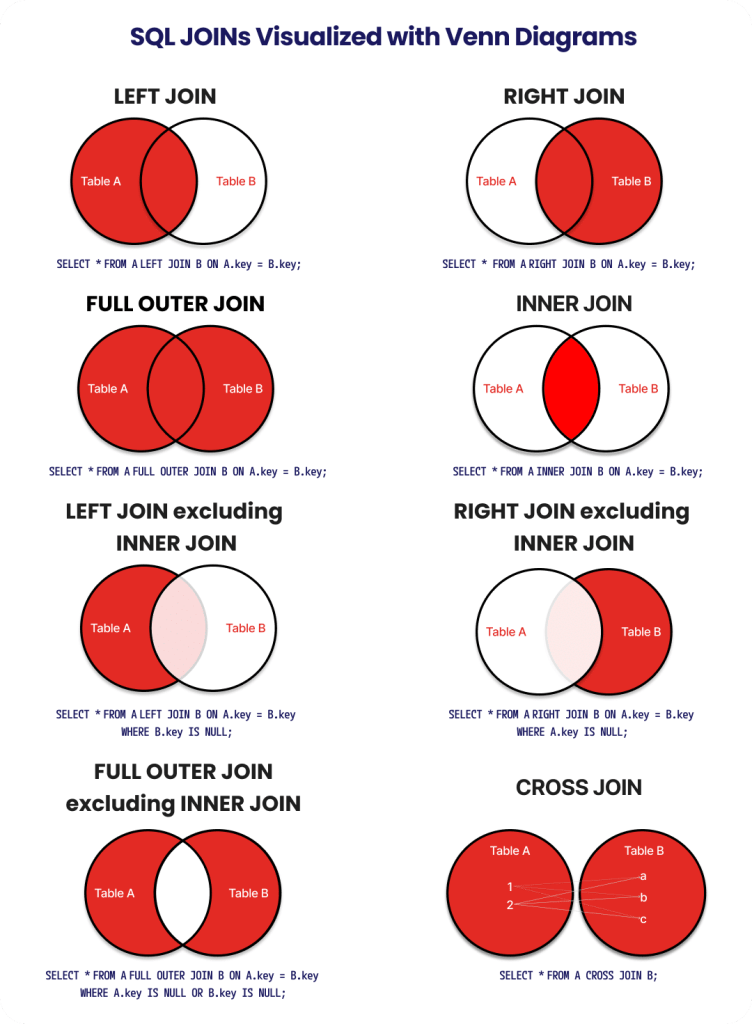
Venn diagrams are a common way to illustrate the basic SQL join types, although they do not show cardinality or fanout. In practice, I have gotten away with using inner and left joins almost exclusively for years. Occasionally, I use an anti-join to exclude existing matches or a cross join to create every combination, such as a complete user-by-date spine.

Semi-structured data adds another complication. One cell can contain its own universe of information. I once worked with a table that stored every hardware setting for every action taken on a device. Imagine saving every toggled setting with every click. That grows quickly.

Packing the payload into JSON can make logging simpler and more flexible for product engineers. For analytics, repeatedly reading and extracting the same fields creates extra work. Frequently used fields can be pulled into typed columns or a smaller downstream model, while the less common details remain in the JSON.

I have noticed that engineers vary in how much they optimize logging for downstream analytics. There is a real tradeoff between making the data convenient for analysts and taking engineering time away from shipping the product. Often, I would rather clean up the JSON downstream and build a small reusable model than ask engineers to perfectly structure every field at the source.

Sometimes when I get stuck, I find I need to solve the problem on paper first with one example before coding it out. For a join, that might mean writing out a few rows from each table and the result I expect. 

Tables, Views, and Pipelines

Say I have worked out my joins and written the final query. The next decision is whether to store the logic or its results.

A view stores the SQL instructions and runs them when someone queries it. The view itself takes up little space and reflects the current state of its sources, but complicated views can repeatedly perform the same expensive work. A table stores the result. It is usually faster to query, but requires storage and must be rebuilt or updated when the underlying data changes. A materialized view sits between the two: it stores a precomputed result that must be refreshed as its sources change.

Materialization mostly determines when I pay the cost. With a view, I pay when someone queries it. With a table, I pay during the scheduled build. This makes tables useful for expensive transformations that are queried repeatedly, while views work well for simpler logic or data that needs to remain current.

A Common Table Expression, or CTE, is a named subquery used inside one larger query. I mostly use CTEs to make SQL readable and break complicated logic into steps. A CTE does not guarantee that its results are stored. The query optimizer may combine it with the rest of the query or temporarily materialize parts of it.

For example, a window function may need to partition and sort a large intermediate result. Turning the CTE into a table can avoid repeating that work across future queries, but it also creates another object that must be stored, refreshed, and maintained. A useful general rule is to materialize expensive or frequently reused transformations and leave simple, single-use logic in CTEs or views.

In dbt, a query can be materialized as a view, table, incremental table, or ephemeral model. Intermediate models isolate reusable transformation steps before they are joined into final models. If I wanted to identify users who use both web and mobile, I might first create a web-user model and an app-user model, then inner join them. If that logic is used only once, two CTEs might be enough. If the same user sets support several models, storing them as intermediate models saves duplicated work and creates one definition that everyone can reuse.

Once transformations are split across models, one query becomes a pipeline, with its dependencies forming a structure known as a directed acyclic graph (DAG). Each model depends on its upstream sources and must wait for them to finish. This makes the logic easier to test, reuse, and understand, but every added dependency creates another possible delay or failure.

I generally want the closest stable upstream model that already owns the definition I need. Going all the way back to raw data can duplicate cleaning and business logic. Depending on a distant downstream model can add unnecessary columns, transformations, and wait time. The best source is usually the simplest trusted model at the right grain.

For very large tables, rebuilding the full history every day can become impractical. An incremental model processes only new or changed data, usually by appending new rows or merging them into existing ones. For a daily snapshot of every loan at a company, I might process the newest date along with a few recent dates to capture late-arriving data.

Incremental models make routine builds much faster, but they introduce more state and logic. They need a reliable way to identify new or changed records, handle updates and duplicates, and recover from missed runs. Their runtime can also vary with recurring changes in data volume, such as weekday versus weekend transaction traffic, which can affect downstream orchestration. Changes to the model’s logic, historical corrections, and major backfills may still require a full rebuild. My earlier issue appeared during one of those rebuilds. The incremental run was fast, but it had hidden how expensive the complete model had become.

A common warehouse flow starts with raw source data, then moves through staging models that rename, type, and clean it. Intermediate models join sources, apply transformations, and change grains. Fact and dimension tables represent stable business concepts. Finally, marts or serving models organize the data for particular teams, dashboards, ML systems, or other consumers.

Every company names and divides these layers differently. I do not need to understand every domain and use case to follow the general flow from raw data toward increasingly structured and specialized models.

What the Warehouse Actually Does

I’m not going to get deeply into clusters and distributed computing, but it helps to understand what happens after I submit a query.

The warehouse first creates an execution plan. Although SELECT is written first, a basic SQL query logically starts with FROM and JOIN, followed by WHERE, GROUP BY, HAVING, SELECT, ORDER BY, and LIMIT. Window functions are calculated after grouping and HAVING but before the final ordering. The optimizer can rearrange the physical work while preserving this logic, deciding which data to scan, which filters to apply early, how to order the joins, and where to aggregate or sort the results. In a distributed warehouse, that work is divided across multiple workers and combined at the end.

Fast queries often come from avoiding work. Columnar storage allows the warehouse to skip columns I did not select. Table statistics and physical organization can help it prune entire sections of data that do not match my filters. This is why filtering a large table can be fast when the relevant data is organized well, but surprisingly slow when the warehouse still needs to scan most of the table.

Analytical warehouses use physical organization such as partitioning and clustering to skip irrelevant data. When these physical layouts degrade or heavy operations spill memory to remote storage, performance drops quickly. Even so, daily query performance usually comes back to the basics: checking join cardinality, selecting fewer columns, and filtering early.

After reading the data, the warehouse may need to move it around. Rows with the same join or grouping keys must reach the same place before they can be combined. Joins, aggregations, sorts, and window functions can all create large intermediate results. If those results do not fit in memory, the warehouse spills them to local or remote storage, which can slow the query considerably.

More compute can divide some of this work across additional workers and provide more memory. It cannot fully rescue a query that scans unnecessary data or creates an enormous intermediate result. Fixing an accidental many-to-many join is usually more valuable than increasing the warehouse size.

Data distribution also factors in. Suppose a table contains 200 million payments and I group them by customer. If the payments are distributed fairly evenly across customers, the warehouse can divide the work across its workers. If one customer accounts for half of all payments, some workers or stages may receive far more work than others. The query then waits for its slowest part to finish. This uneven distribution is called skew. It can slow joins, aggregations, window functions, and incremental builds even when the total row count looks reasonable. Checking the largest groups before a major join or aggregation can reveal this quickly. Skew often comes from an unusually large customer, but it can also hide in default values such as unknown or an empty string.

Finally, production performance includes more than the query itself. Other workloads may be running concurrently, the warehouse may need to start up, and queries may wait in a queue. Cached data or results can make repeated runs appear faster. BI tools can generate inefficient SQL. Tables grow, schemas change, late data arrives, and occasional backfills process much more history than the daily workload.

A local tool like DuckDB is useful for isolating individual effects under controlled conditions. Snowflake exposes the operational reality of shared workloads, caching, warehouse size, and cost. Synthetic tests can teach me why something is slow, but production tells me whether it is actually a problem.

Databases and Data Warehouses

I have worked with several systems that store and query data, but they were designed around different workloads. Postgres and MySQL are commonly used as row-oriented transactional databases, where applications frequently read or update individual records.

Vertica, Redshift, Snowflake, and BigQuery are distributed analytical warehouses built to scan and aggregate large datasets. With the Vertica and Redshift clusters I used, everyone shared a limited pool of compute, so performance declined as more people and pipelines piled on. Snowflake made scaling much easier by separating storage from compute and allowing teams to resize or isolate their warehouses. That flexibility can become expensive if the compute is not managed carefully, but it is also a major reason Snowflake has become so common. BigQuery manages most of the infrastructure serverlessly.

Databricks uses a lakehouse model. A data lake stores large amounts of raw and structured data as files, usually in relatively inexpensive object storage. A lakehouse adds warehouse-like tables, reliability, governance, and query performance on top of that data. This allows SQL, data engineering, and ML workloads to operate on the same underlying data instead of maintaining separate copies across several systems.

Other databases are more specialized. ClickHouse is a columnar analytical database built for fast queries over high-volume data such as events and logs. DuckDB brings a columnar analytical engine into a local process, making it useful for exploration and controlled testing. Turbopuffer specializes in vector and full-text search rather than general warehouse analytics. Vector search converts information such as text or images into numerical vectors that represent their meaning or features. Items with nearby vectors are treated as similar, making this useful for finding relevant documents to supply as context to an LLM.

The important question is what work I need the system to do: transactional updates, large batch analysis, interactive dashboards, local exploration, or search.

Diagnosing a Slow Query

Start With the Workload

Calling a table slow is only the beginning. First, I need to define what is actually failing. Is this a transactional lookup or an analytical query? Is one query slow, or is it a dbt build, dashboard, or entire warehouse? Does it happen consistently, or only when other workloads are running?

The goal also changes what counts as slow. A scheduled model that takes 20 minutes might be acceptable, while a dashboard that takes 20 seconds may be unusable. I might be optimizing for latency, cost, freshness, or the number of queries that can run concurrently. Improving one does not always improve the others.

Consistent slowness usually points toward the query or data model. Intermittent slowness may come from queueing, warehouse startup, competing workloads, caching, or data skew. Comparing a slow run with a normal one is often more useful than examining it alone.

Query Plans and Profiles

In Snowflake, I can start with Query History. It shows how long the query took, which warehouse ran it, how many bytes it scanned, and how many rows it returned. I can also separate time spent executing from time spent waiting in a queue. If execution is fast but the query waits several minutes to begin, rewriting the SQL may not solve the problem.

The query profile breaks the work into operators such as scans, joins, filters, aggregations, sorts, and window functions. I do not need to understand every symbol immediately. I can start with the most expensive operator, then follow how many rows enter and leave each step.

If a table scan dominates, I can look at bytes scanned and partitions scanned versus pruned. A query that returns a small result after scanning most of a large table may need a better filter, fewer columns, or better organization around commonly filtered fields. In Postgres or MySQL, an index can help locate matching rows without scanning the full table, at the cost of additional storage and maintenance. In Snowflake, a clustering key can provide that organization and help the warehouse prune more micro-partitions.

If a join suddenly produces far more rows than it receives, I can check the grain, key uniqueness, and join conditions. Large redistribution or shuffle can point toward an expensive join or skewed key. When estimated and actual row counts are available, a large difference can also mean the optimizer misunderstood the data distribution.

Aggregations, sorts, and window functions often become expensive because they must hold or rearrange large intermediate results. Local or remote spill means those results exceeded available memory and had to be written elsewhere. Filtering, selecting fewer columns, aggregating earlier, or materializing a reusable step can reduce that work. Increasing compute may help when the work itself is legitimate but too large for the current warehouse.

Finally, I compare the rows returned with the work performed. Returning millions of rows can be slow even when the query plan is reasonable. Often the answer is simply to ask a narrower question and tailor it more to the demand.

For my original incremental model, I could compare the normal incremental run with the much more expensive full rebuild. The incremental version scanned only recent data, while the rebuild exposed the cost of processing the entire history. Incrementality had made the daily workload manageable, but it had also hidden how expensive the complete model had become.

Putting It to the Test

I ran some local DuckDB experiments to see how several basic modeling choices affect query performance. Increasing a table from 100,000 to 100 million rows added 1,000 times as many rows but took 144 times as long to query. Reading 25 columns instead of one took 16 times as long. Randomly ordered data took 5.6 times as long as data sorted by the filtered date, while a join producing five matches per key took 4.6 times as long as a one-match join. Finally, rebuilding 10.1 million rows took 37 times as long as appending 100,000 new rows.

These are educational demonstrations, not production benchmarks. Each experiment changed one major variable and used one warm-up followed by 10 measured runs. Relative runtimes should only be compared within each experiment.

Row Count

Rows	Median runtime	Relative runtime
100K	0.19 ms	1.0×
1M	0.43 ms	2.2×
10M	2.43 ms	13×
30M	7.15 ms	38×
100M	27.41 ms	144×

Increasing the table from 100,000 to 100 million rows added 1,000 times as many rows but took about 144 times as long to query. Row count clearly mattered, but it was not a direct proxy for runtime across the full range. At larger sizes, the relationship was much closer: moving from 10 million to 100 million rows increased the row count 10 times and query time about 11 times (GitHub).

Columns Read

Columns read	Median runtime	Relative runtime
1	4.50 ms	1.0×
5	15.94 ms	3.5×
25	73.92 ms	16×

Reading 25 columns took about 16 times as long as reading one. Each query returned only a few aggregates, so the experiment measured reading and processing the columns rather than transferring or displaying millions of rows (GitHub).

Physical Organization

Organization	Median runtime	Relative runtime	Eligible row groups	File size
Sorted by date	1.22 ms	1.0×	3/82	49.3 MB
Random order	6.83 ms	5.6×	82/82	98.5 MB

Both files contained the same 10 million logical rows and returned the same 191,779 matching rows. In the sorted file, only 3 of 82 row groups had date ranges that overlapped the filter. All 82 were eligible in the randomly ordered file. The sorted file was also half the size, so the result reflects both better pruning and better compression (GitHub).

Join Cardinality

Matches per key	Output rows	Fanout	Median runtime	Relative runtime
1	10M	1×	25.17 ms	1.0×
5	50M	5×	116.80 ms	4.6×

Joining the fact table to one dimension row per key produced 10 million rows. Allowing five matches per key produced 50 million rows and took about 4.6 times as long. A join does not merely add columns; its cardinality determines how many rows must be processed afterward (GitHub).

Incremental Build

Build strategy	Rows processed and written	Final rows	Median runtime	Relative runtime
Incremental append	100K	10.1M	2.39 ms	1.0×
Full rebuild	10.1M	10.1M	88.23 ms	37.0×

Both approaches produced the same verified 10.1-million-row target. Rebuilding the complete table took 37 times as long as appending one new date. This was a simple append-only example and does not cover merges, updates, deletions, late corrections, or schema changes (GitHub).

Methodology and Limitations

The benchmarks ran locally using DuckDB 1.4.5 and Python 3.9.6 on an Apple Silicon Mac with eight logical CPUs and 16 GiB of memory. Absolute runtimes will vary across computers. The more useful result is how performance changed within each controlled experiment. Local DuckDB also cannot reproduce distributed-worker skew, warehouse congestion, concurrent workloads, or the operational behavior of systems such as Snowflake and BigQuery (GitHub).

AI, Data, and Judgment

LLMs are very good at writing SQL, but they do not escape the computational reality underneath it. The warehouse still has to scan the data, execute the joins, move intermediate results, and return an answer. AI can generate a query instantly that takes hours to run.

AI also lets me work faster in unfamiliar domains, sometimes without learning the underlying models as deeply. It keeps me from getting bogged down in writing code and searching for context, but it can also tempt me to skip steps. The faster I move, the easier it is to make mistakes if I rely on it without validating the result.

It is a little like driving instead of running. The car gets me farther, faster, but when it breaks down, I still need to understand how it works well enough to diagnose the problem. Moving faster makes judgment more important. I still need to clarify the question, understand the grain, validate the joins, and recognize when the result or runtime looks wrong.

Wrap Up

I have always seen data models as a means to an end: producing reliable information that improves decisions. This post was my attempt to build a deeper understanding of what happens underneath.

Thanks to Manoj Krishnan, Dina Jankovic, Kasia Rachuta, and Rob Wang for the review!